
Tensorflow: AI 101
Learn how to build basic machine learning AI models.
Tensorflow: Build Machine Learning Models
This week includes challenges about how to design, test, and build machine learning models with Tensorflow. Tensorflow can be thought of as a layer of software that abstracts away a significant amount of the low level programming (CUDA, C), while allowing the individual layers and traning models to be done. This is a good way to think about the position of Tensorflow:
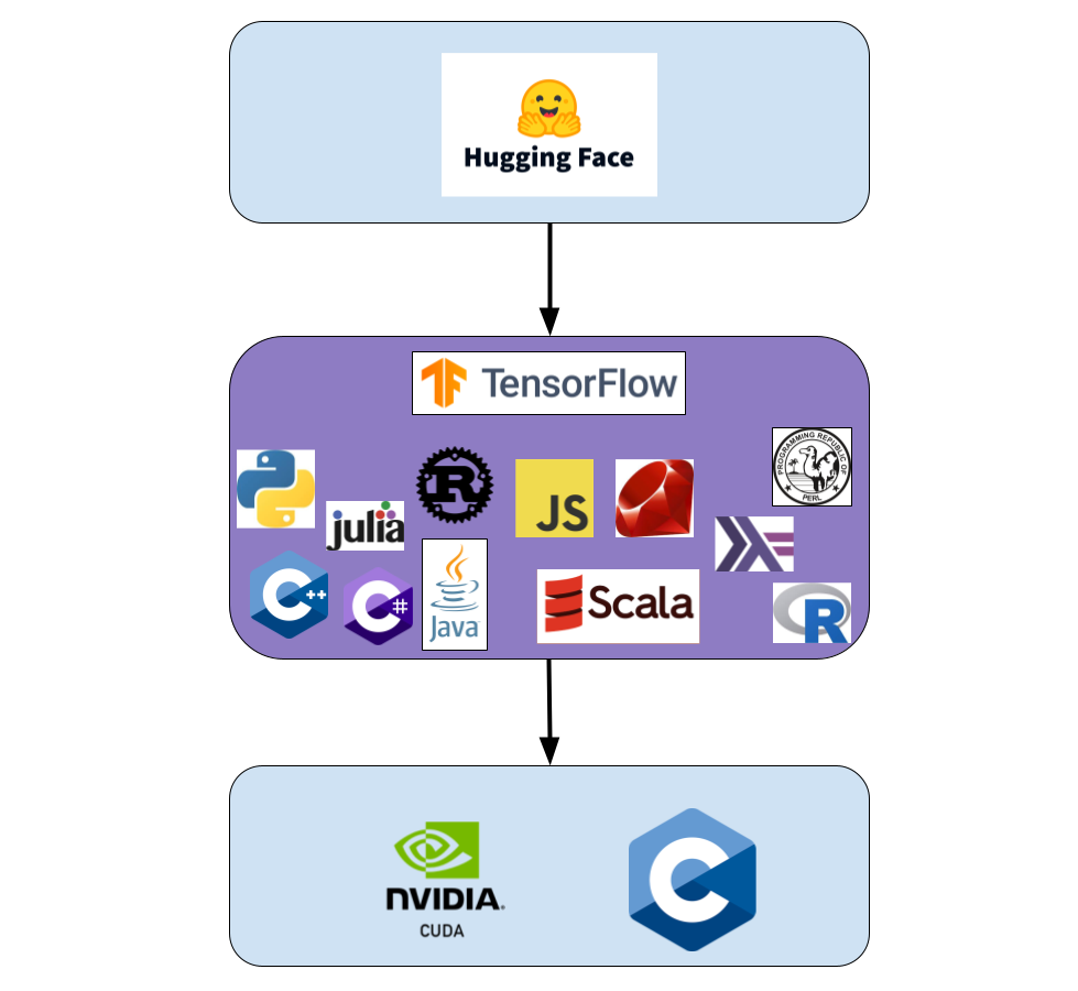
Tensorflow is a common framework that is written to be used in a wide variety of languages. It is supported by underlying software and CUDA (if your system has GPU that uses CUDA). Tensorflow can also be used in conjunction with other models from a place such as Hugging Face, and can even be used to build models that can be hosted and shared on a platform such as Hugging Face. Also, yes, these are all languages that receive official TensorFlow support.
Now, into the basics of machine learning you should understand before we engage in creating some models!
What is a tensor?
A tensor is a matrix. It contains a set of values that are shaped into a box, with unique properties. A tensor comes in all shapes and sizes. Tensors are used in both graphics and machine learning. Matrix operations have been heavily optimized on modern GPUs, which is beneficial for machine learning, as these models can be easily represented as a series of tensors, which allows models with hundreds of thousands of weights to quickly process results and make predictions.
Tensor examples:
$$\begin{bmatrix} 1 & 2 & 3 & 4 & 5 \end{bmatrix}$$
$$\begin{bmatrix}
1 \\
2 \\
3 \\
4 \\
5
\end{bmatrix}$$
$$\begin{bmatrix} 2 & 4 & 6 & 8 & 10 \\ 1 & 3 & 5 & 7 & 9 \end{bmatrix}$$
$$\begin{bmatrix} 1 & 0 & 0 \\ 0 & 1 & 0 \\ 0 & 0 & 1 \end{bmatrix}$$
What is a machine learning model?
You can imagine a machine learning model as several layers that all perform basic operations on a tensor. There are several different operations depending on the layer. The most common layer is a Dense/Fully Connected layer. In this layer, every node is the sum of every node in the previous layer, multiplied by a weight, and added to a bias.
In a more mathematical notation, one output node can be represented by:
$$(\Sigma^{n}_{i=0} w_i * x_i) + b$$
Or, with matrices, all output nodes can be represented as follows:
$$W \cdot \vec{x} + \vec{b}$$
In a more visual sense here is a image of what this layer ends up looking like:
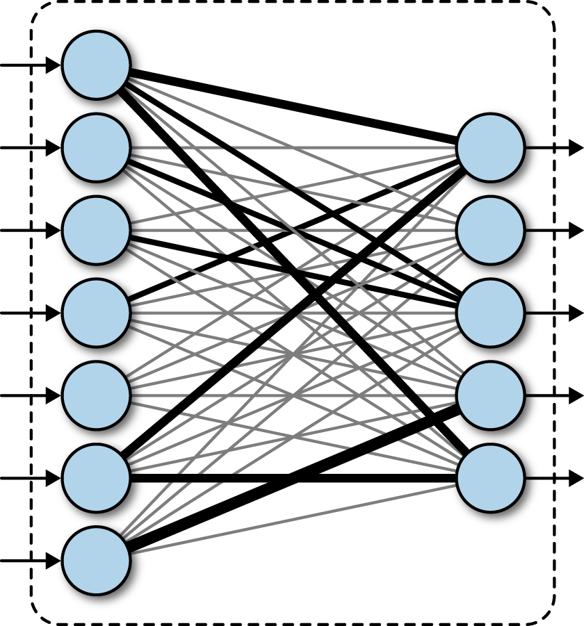
These layers, along with several other layers, form the basic backbone of a neural network. The only step missing is that there is usually an “activation” function applied to a node. This ensures values do not scale out of control, and all weights have the oppurtunity to impart their own influence without certain sections of the network dominating the output.
There are a few more important aspects of a machine learning model:
- Forward Function: This function will pass an input through the network (ie. Calculating the weights associated with each node), and return the outputs in the final nodes.
- Loss Function: This function will take in the output of the model for a given input, along with the expected output and calculate a value representing how well the model did. This forms the basis of training, as it determines the difference between the current model state and what the output should be.
- Optimization Function: This function takes in the loss function output, and calculates the best method for adjusting the weights and biases of the models to reduce the loss (the difference between expected and real outputs). An optimization is designed to treat the loss function as the output of a function that takes in all of the weights and biases of the model. The optimization function attempts to find the minimum value of loss by taking “steps” to adjust the weights and biases that are the inputs.
- Backward Function: Applies all of the optimizations calculated by the optimization function to the weights in the model.
- Batches: A method for performing optimizations more frequently by only using a portion of the training set, without needing to process the entire set before calculating the loss and optimization before applying them.
- Hyperparameters: Variables that influence the model. The most significant is the learning rate, that determines the magnitude of the changes that the optimization function can apply to the weights and biases.
Now! To real programming!!
Python & Tensorflow
Python is the easiest library to use with Tensorflow for a few reasons:
- Python is a simple, easy to write language
- Python has existing libraries that make it significantly easier to perform data calculations, include Numpy, Pandas, CSV processing, built-in dictionaries, and MatPlotLib.
- Python also has the entire SciPy tool suite, including scikit-learn, which provides simpler, built-in predictive models that can be used to solve simpler correlation and relation problems.
Additionally, Google provides “Google Colab”, which is a method for running Python code, with Tensorflow, directly on a free server with GPU support. For all of these challenges, you can complete them in Google Colab.
Finally, here is a quick disclaimer. Tensorflow’s Keras library is responsible for the high level abstractions. We will be almost exclusively using this library for all of the challenges.
Documentation:
Tensorflow Tutorials
Tensorflow Keras Python Docs
Google Colab
Easy Challenges (100 points):
Matrix Math (50 points):
Using only Tensorflow, write a script that performs the following operations:
-
Create a 3 x 3 matrix that contains random contents in the range of 1 to 9. Hint: Your code should resemble the following:
x = tf.random.uniform(???, minval=???, maxval=???) print(x) -
Multiply the random matrix by another matrix, such that the result is the same random matrix.
# This is the identity property of a matrix; ie. A x I = A. What should I be? Note: This is matrix multiplication, not bitwise multiplication A = tf.random.uniform(???, minval=???, maxval=???) I = ??? R = # A times I print(R) -
Create a 7 x 5 matrix of all 0’s, and use a loop to set all of the elements to be 5.
A = # Create a 7 by 5 array of all 0's for x in range(???): for y in range(???): A[???] = 5 -
Calculate the outputs of a basic fully-connected layer that takes in five inputs and returns two outputs. The weights and biases should be uniformly random, in the range of 0 to 1, but the inputs should be [1, 2, 3, 4, 5]
    X = tf.constant([[1, 2, 3, 4, 5]], dtype=float)
    X = tf.transpose(X)
    W = # Create uniform array with dimensions (2, 5)
    b = # Create uniform array with dimensions (2, 1)
    output = # W x X + b
    print(output)
MNIST Basics (50 points):
Now, it is time to do the most common introduction neural network: Image classification with the MNIST dataset. Below is the starter code:
First block:
    import tensorflow as tf
    from tensorflow import keras
    from tensorflow.keras import layers

    from tensorflow.keras.datasets import mnist
    (x_train, y_train), (x_test, y_test) = mnist.load_data()

    print(x_train.shape) # Should output (60000, 28, 28)
    print(y_train.shape) # Should output (60000,)

    # Reshape into 60000 samples of 1-D arrays and normalize in the range (0-1)
    x_train = x_train.reshape(-1, 28*28).astype("float32") / 255.0
    x_test = x_test.reshape(-1, 28*28).astype("float32") / 255.0

    print(x_train.shape) # Should now output (60000, 784)
Second block:
    # Input layer should take in an array of (28*28, )
    # First hidden layer should have 512 inputs and use the "relu" activation function
    # Must classify outputs into being a value in the range (0-9)
    # Adam optimizer should use a learning rate of 0.001

    inputs = keras.Input(shape=(???, ))
    x = layers.Dense(???, activation=???)(inputs)
    x = layers.Dense(256, activation="relu")(x)
    outputs = layers.Dense(???, activation="softmax")(x)
    model = keras.Model(inputs=inputs, outputs=outputs)

    model.compile(
        loss=keras.losses.SparseCategoricalCrossentropy(from_logits=False),
        optimizer=keras.optimizers.Adam(learning_rate=???),
        metrics=["accuracy"]
    )

    model.fit(x_train, y_train, batch_size=32, epochs=5, verbose=2)
    model.evaluate(x_test, y_test, batch_size=32, verbose=2)

    # Write a print statement that will display: "The evaluation showed the model had an accuracy of {accuracy_output}%"
Third block:
    import matplotlib.pyplot as plt
    import numpy as np
    (x_train_images, _), (x_test_images, _) = mnist.load_data()


    # Change 700 to any value in the range 0 to <60,000
    image = x_train_images[700]
    image_eval_data = image.reshape(-1, 28*28).astype("float32") / 255.0


    plt.imshow(image, cmap="gray")
    plt.show()

    predictions = model.predict(image_eval_data)
    predicted_class = np.argmax(predictions[0])

    print(f"The predicted class for the custom image is: {predicted_class}")
When this is filled in correctly, you should have a working model with a high accuracy that you can use to test against different inputs to the function. Be certain the final accuracy is greater than 95%, and test with a wide range of different images.
Medium Challenges (100 points):
Convolutional Neural Network Basics (100 points)
Convolutional neural networks are a method of processing image data in a way that can more effectively understand the contents of the image. The main ideas of convolutional neural networks is that they can find features in an image and highlight these features. How would this work?
What is a convolution?
A convolution is pretty simple. Here is a basic example of a 5 x 5 image that contains a 7-like shape:
$$\begin{bmatrix}1 & 1 & 1 & 1 & 1 \\ 0 & 0 & 0 & 1 & 0 \\ 0 & 0 & 1 & 0 & 0 \\ 0 & 1 & 0 & 0 & 0 \\ 1 & 0 & 0 & 0 & 0\end{bmatrix}$$
This is a simple grayscale, small image. Now, a convolution will have a random pattern (initially). To make this demonstration easier, we will only look at one convolution that is 3 x 3 and only contains 1s:
$$\begin{bmatrix}1 & 1 & 1 \\ 1 & 1 & 1 \\ 1 & 1 & 1 \end{bmatrix}$$
There will also be a bias included with the convolution. We will also just use a bias of 1.
Now, the convolution can be applied by “sliding” our convolution matrix across our image matrix, and performing element-wise multiplication and adding the bias. Applying this matrix results in the following output:
$$\begin{bmatrix}5 & 6 & 6 \\ 3 & 4 & 3 \\ 4 & 3 & 2\end{bmatrix}$$
Note that even with a bad, single convolution, the heaviest values still form the shape of the initial 7.
Additionally, how this really works in a convolutional neural network is that the initial 7 would be duplicated several times (lets say 128), creating a 5 x 5 x 128 matrix, that would then be iterated through by a 3 x 3 x 128 matrix, where each 3 x 3 matrix is randomized, and then trained using traditional optimizers.
After several convolutions are applied, eventually, the output is flattened into a linear layer, that can be passed into a traditional, fully connected neural network, and classified.
One final thing to note is that there are other layers needed for a convolutional neural network. The most common are MaxPooling layers, that perform a convolution that takes the maximum of a section of a matrix. A simple example is to use this matrix:
$$\begin{bmatrix}1 & 2 & 5 & 6 \\ 3 & 4 & 7 & 8 \\ 9 & 10 & 13 & 14 \\ 11 & 12 & 15 & 16\end{bmatrix}$$
Now, applying a 2 x 2 max pooling layer will slide a 2 x 2 matrix across the matrix and take the maximum of the captured matrix. Additionally, by default, the “slide” amount (called stride) will be equal to the size of the pooling layer. Applying a 2 x 2 max pooling layer will result in the following:
$$\begin{bmatrix}4 & 8 \\ 12 & 16\end{bmatrix}$$
This will ensure the most relevant details are saved, while reducing the computational load.
Create a convolutional neural network (100 points)
For this challenge, all you need to do is fill in sections of this code and run the training model.
Block 1
import tensorflow as tf
from tensorflow import keras
from tensorflow.keras import layers, regularizers

from tensorflow.keras.datasets import cifar10

(x_train, y_train), (x_test, y_test) = cifar10.load_data()

x_train = x_train.astype("float32") / 255.0
x_test = x_test.astype("float32") / 255.0

print(x_train.shape)
Block 2
# What should the input shape be for the data??
# All of the max pooling should be for a 2 x 2 matrix (Note: Tensorflow helps out, as every MaxPooling2D will be the same size after initial declaration)
# How is the Cifar10 dataset classified? What are the number of outputs? Be certain to create a layers.Dense layer with the number of possible outputs
model = keras.Sequential(
    [
        keras.Input(shape=(???)),
        layers.Conv2D(128, (3, 3), padding='valid', activation='relu'),
        layers.MaxPooling2D(???),
        layers.Conv2D(256, (3, 3), padding='valid', activation='relu'),
        layers.MaxPooling2D(),
        layers.Conv2D(1024, (3, 3), padding='valid', activation='relu'),
        layers.MaxPooling2D(),
        layers.Flatten(),
        layers.Dense(64, activation='relu'),
        # Output layer,
    ]
)

model.compile(
    loss=keras.losses.SparseCategoricalCrossentropy(from_logits=True),
    optimizer=keras.optimizers.Adam(learning_rate=3e-4),
    metrics=["accuracy"],
)

model.fit(x_train, y_train, batch_size=64, epochs=10, verbose=2)
model.evaluate(x_test, y_test, batch_size=64, verbose=2)
Block 3
import matplotlib.pyplot as plt
import numpy as np
(x_train_images, _), (x_test_images, _) = cifar10.load_data()

# What are the potential classifications (in order) for the given dataset?
classification_array = [???]


image = x_train_images[700]
image_data = image.reshape(-1, 32, 32, 3).astype("float32") / 255.0

plt.imshow(image)
plt.show()

predictions = model.predict(image_data)
predicted_class = np.argmax(predictions[0])

print(f"The predicted class for the custom image is: {classification_array[predicted_class]}")
These are this week’s challenges! Be certain to talk to an officer if you want more guidance or to submit the challenge. You can also use the submission Google form to submit your answer.